Imagine you work as an AI developer and your team has trained an image classification model. The validation and testing step was successful and your model shows a pretty good accuracy, precision and recall; let’s say about 0.98, 0.97 and 0.99, respectively. Great. However, the model has to make important decisions based on its own predictions, with no human supervision. Your model is fine, but just like any other neural network it looks like a black-box, and both you and your team cannot explain why it returns those predictions, even if they are correct.
This raises a serious trust issue, because no one can ensure that in certain never-before-seen situations the model will continue to perform properly. The interpretability of the model’s decisions is lacking and you need to understand why it makes certain decisions given certain inputs. For this reason, a new research topic called Explainable AI (XAI) has been emerging. Its aim is to find methods to investigate model outputs against their inputs.
From an image perspective, classifications based on Convolution Neural Networks are the best candidates for this purpose.
There are essentially two categories of approach: model-agnostic techniques and model-based methods. The first ones include methodologies that can be applied to any type of model, whether it is a neural network or a classic machine learning algorithm, since they only need inputs and outputs and do not require access to model internals (like hidden layers, weights, biases etc.). The last ones includes a set of techniques that need to act directly on model internals (e.g., computing gradients).
Let’s look at some of them.
LIME
LIME stands for Local Interpretable Model-agnostic Explanations, and thanks to the use of local interpretable features, it helps to identify key features that influence the output of a given model, allowing for an enhanced understanding of the decision-making process of a given model. When dealing with images, local features refer to specific shapes, with specific colors or textures. The presence or the absence of those features modify the output of the classification in such a way that can be observed to understand the model behaviour. In a nutshell, the following steps are performed:
1. Superpixel Segmentation: a computer vision technique to divide image in multiple pieces that share same local properties. Each superpixel is a local feature. The result could be the one to the right:

Credits: Aditya Bhattacharya towardsdatascience.com
2. Masking Inference: the image is fed to the classification models multiple times but each time randomly turning off some superpixels (black color) and keeping on others. The results are a set of prediction rankings based on slightly different input images.
3. Computing Local Feature Importance: an algorithm computes the weight of each superpixel that contributes to each class scores. An heatmap is generated as below: it highlights very well the importance of the foreground shark for the prediction output class “Shark”.
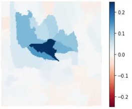
Credits: Aditya Bhattacharya towardsdatascience.com
In this way it is possible to understand what the model is looking at. It may in fact happen that the model gives the correct prediction but focuses on wrong features (such as the sand in the example before).
Occlusion Method
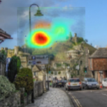
This model-agnostic method is both very simple and effective. It consists of submitting the same image to the model many times, occluding or blurring specific parts of the image for each trial. By doing this, each iteration perturbs different part of the image several times. The intuition behind this approach is that classification should change dramatically when an important region is occluded. In contrast, the occlusion of pixels that have minimal impact on the classification scores and are therefore less important, should not should affect the result. After this procedure, a saliency map is created. This map is usually generated in the form of a heat map, highlighting the most important pixels, thus showing which pixels most influenced the network decision to yield a specific class.
An example of iterations and outputs:
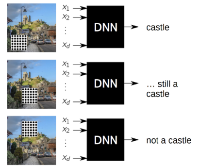
Credits: Aditya Bhattacharya towardsdatascience.com
Grad-CAM
Grad-CAM stands for Gradient-weighted Convolution Activation Mapping and it is a model-based method with the purpose of projecting onto the input image the regions responsible for maximum activation of a specific class. For this reason, unlike previous techniques, it requires access to the hidden layers of the model (particularly convolutional layers) up to Global average pooling. The approach is as follows: the method uses the gradient information in the last convolutional layer of the model to understand the contribution of each neuron with respect to a class of interest.
To obtain the class discriminative localization map for any class C, the gradient of the score for the class C before the SoftMax is computed with respect to feature maps Ak of a convolutional layer. These gradients flowing back are global average-pooled to obtain the neuron importance weights Ak for the target class. After calculating Ak for the target class C, a weighted combination of activation maps followed by ReLU activation is performed. The result is an heatmap of the same size as that of the convolutional feature maps projected onto the original image, indicating the most important regions that activate the specific output.
An example is shown below: the original image, the activation map for class “Dog” and the projected saliency map.

Credits: Divyanshu Mishra
Conclusions
The approaches analyzed in this article are only some of the most widely used. Explainable AI is an ongoing field with the aim of demystifying the black-box aspect of AI models. It should be mentioned that model-agnostic techniques generally have the shortcoming of being less accurate and requiring a longer runtime than techniques that have access to model internals and dynamics.
This article has been written by Giovanni Nardini – R&D Artificial Intelligence Lead
